
Vorticity Analysis
The vorticity [1] is defined to describe the rotation of the fluid particles and in 2D, it is expressed as

where v is the velocity in horizontal direction and u is the velocity in vertical direction. The vorticity can either be positive or negative, which indicate the direction of rotation.
In Figure 1, the height of the leading edge vortex at angle of attack 2° is equivalent to 7 grid rows and the length is equivalent to 14 grid columns. The centre of the leading edge vortex can be considered as in the 7th grid column. The profile of the vorticity in the 7th column is shown in Figure 2. From the profile for the 7th grid column, the peak vorticity appears in the 15th grid row. The high vorticity area is above the leading edge vortex (see brown curve). And the vorticity inside the leading edge vortex is relatively small, which means that the leading edge vortex tends to be irrotational.
In Figure 1, the height of the leading edge vortex at angle of attack 2° is equivalent to 7 grid rows and the length is equivalent to 14 grid columns. The centre of the leading edge vortex can be considered as in the 7th grid column. The profile of the vorticity in the 7th column is shown in Figure 2. From the profile for the 7th grid column, the peak vorticity appears in the 15th grid row. The high vorticity area is above the leading edge vortex (see brown curve). And the vorticity inside the leading edge vortex is relatively small, which means that the leading edge vortex tends to be irrotational.
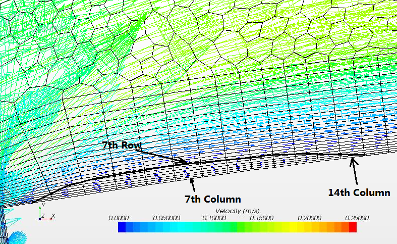
Figure 1:Velocity Vectors near the Leading Edge
|

Figure 2:Contours of Vorticity near the Leading Edge
|
The vorticity can be produced, dissipated or convected to the surrounding. For incompressible viscous flow at constant density in the simulations of this project, it obeys the vorticity transport equation [2] which is expressed as

Where v is the kinetic viscosity of the fluid and u and v are the velocity in horizontal and vertical directions. For simplification, the five terms are represented using A, B, C, D and E in sequence. The first term A is the vorticity change rate against time. Term B and C mean the convective transport of the vorticity in the horizontal and vertical directions separately. Term D and E represents the production and dissipation of vorticity due to viscosity. The vorticity transport equation can be simplified below as term A and D are observed to be small in scenes in Star-CCM+.

This equation indicates that the vorticity produced (term E) is convected to the surroundings (term B and C) and dissipated in different areas when the term E changes the sign.
Vorticity Change on the Leading Edge
Figure 3 and Figure 4 are the illustrations of the term E and term B+C with the grids as a reference of location. The scalar fields are unified from -200 to 200 (see the colour bars in Figure 3 and 4). The white areas in the figures indicate that the values there exceed the maximum or minimum values in the colour bar and cannot be represented by any colours. Whether the white area has large values or small values can be inferred from the surroundings. For example, in Figure 3, the area tagged as positive is surrounded by the red colour, which means the values are high in this area and vice versa for the area with the negative sign.

Figure 3:Contours of Production and Diffusion of Vorticity due to Viscosity
|

Figure 4:Contours of Convective Transport of the Vorticity
|
The figures can be used to understand the vorticity production and dissipation mechanism. From Figure 3, it can be seen that there are three layers from up to down. In the upper layer and the lower layer (denoted using the negative signs), term E is negative meaning that the vorticity is being dissipated, while in the middle layer, the vorticity is being produced as tagged with the positive sign. Figure 4 shows the scene of term B+C. The situations correspond to that in Figure 3, which shows that the vorticity produced in the middle layer is convected to the surroundings. Thus the system is a conserved state. It further proves the validation of vorticity transport equation.
Vorticity Change on the Middle of the Plate Surface

Figure 5:Contours of Vorticity over the Middle of the Surface
The vorticity over the middle of the surface is generally small and has little variation in the vertical direction as shown in Figure 5.
Severe vorticity production and dissipation gradually fade away as in Figure 6, the white areas surrounded by both blue and red colours narrow down when flow goes downstream. The production and dissipation of vorticity happens more obviously in a distance from the aerofoil surface leaving the area near the surface a region of both low vorticity and low vorticity changing. The similar situation for the vorticity convection is shown in Figure 7. |

Figure 6:Contours of Production and Diffusion of Vorticity due to Viscosity

Figure 7:Contours of Convective Transport of the Vorticity
|
Reference
[1] Douglas, Gasiorek and Swaffield. (1995). Rotational and Irrotational Flow. Two-Dimensional Ideal Flow. Fluid Mechanics. 3rd edition. New York: Longman. p191-193.
[2] F.Kaplanski. The vorticity equation and its applications. Tallinn University of Technology. Online Available: <http://www.google.co.uk/url?sa=t&rct=j&q=&esrc=s&source=web&cd=3&cad=rja&uact=8&ved=0CEEQFjAC&url=http%3A%2F%2Fwww.brighton.ac.uk%2Fshrl%2Fshrl%2Fevents%2FThe%2520vorticity%2520equation%2520and%2520its%2520applications.ppt&ei=V7tPU6aSJsP17Aax8YC4Bg&usg=AFQjCNHy_-EMgpbieSBVUeiE_d0_pJsR_g&sig2=2MIBSEXSOeZQMa1LIFmDIQ&bvm=bv.64764171,d.ZGU>. Last accessed 7th May 2014.
